Return to Introduction
Return to Observing Objectives
Return to Mission Technology

Interplanetary Magnetic Field

Cranfill Effect
Global MHD Model Predictions / Voyager 2 Observations
Field Direction Fluctuations
Reconnection
Return to Interstellar Probe Introduction
Return to Observing Objectives


Interplanetary Magnetic Field in the Inner Heliosheath

The Heliospheric Magnetic Field

(also known as "The Interplanetary Magnetic Field" or IMF)


The  magnetic field of the Sun is carried outward by the solar wind. Because the Sun rotates, the field is drawn into Archimedian spirals. These spirals are shown here, for three magnetic field lines at solar latitudes of 6, 45, and 84 degrees north (green, orange, and red, respectively). 

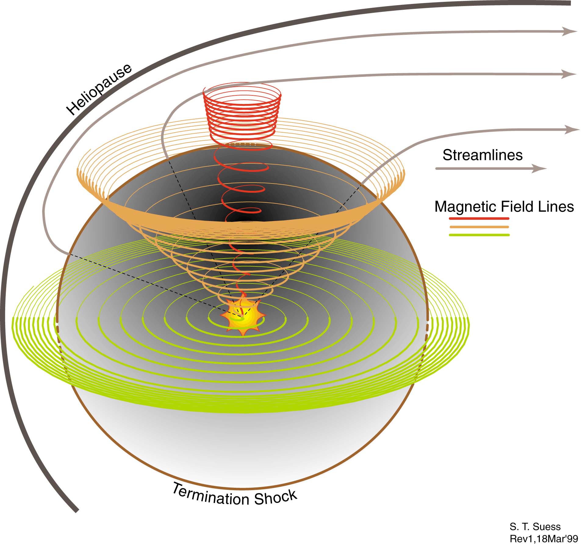
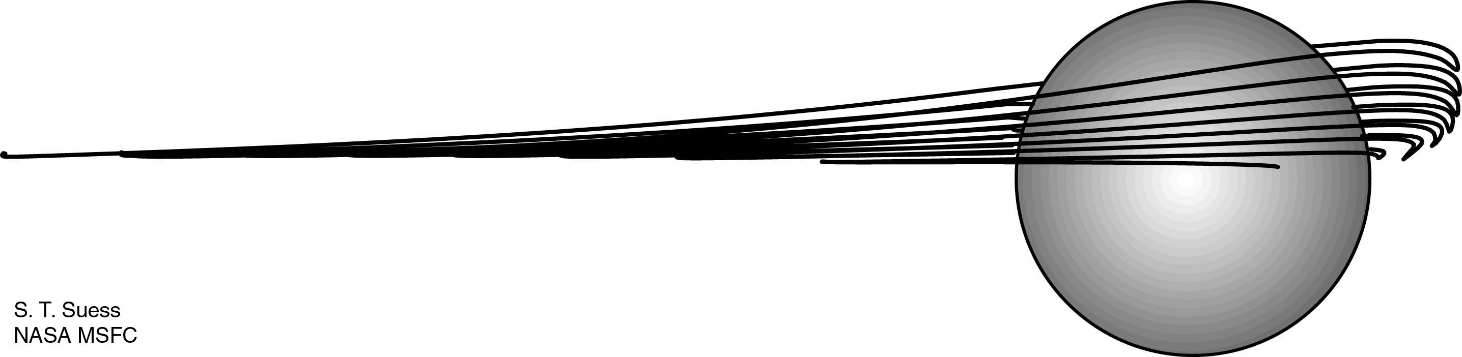
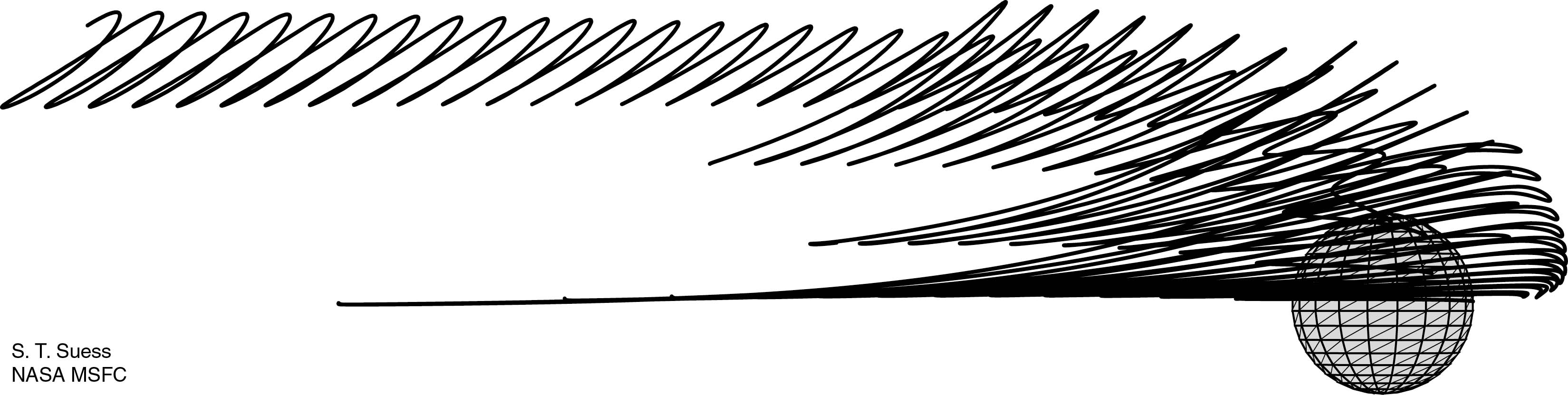
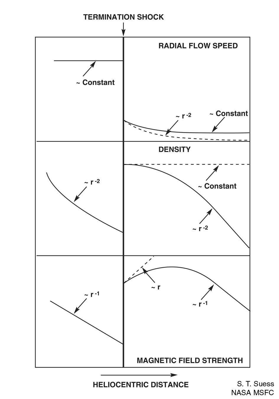
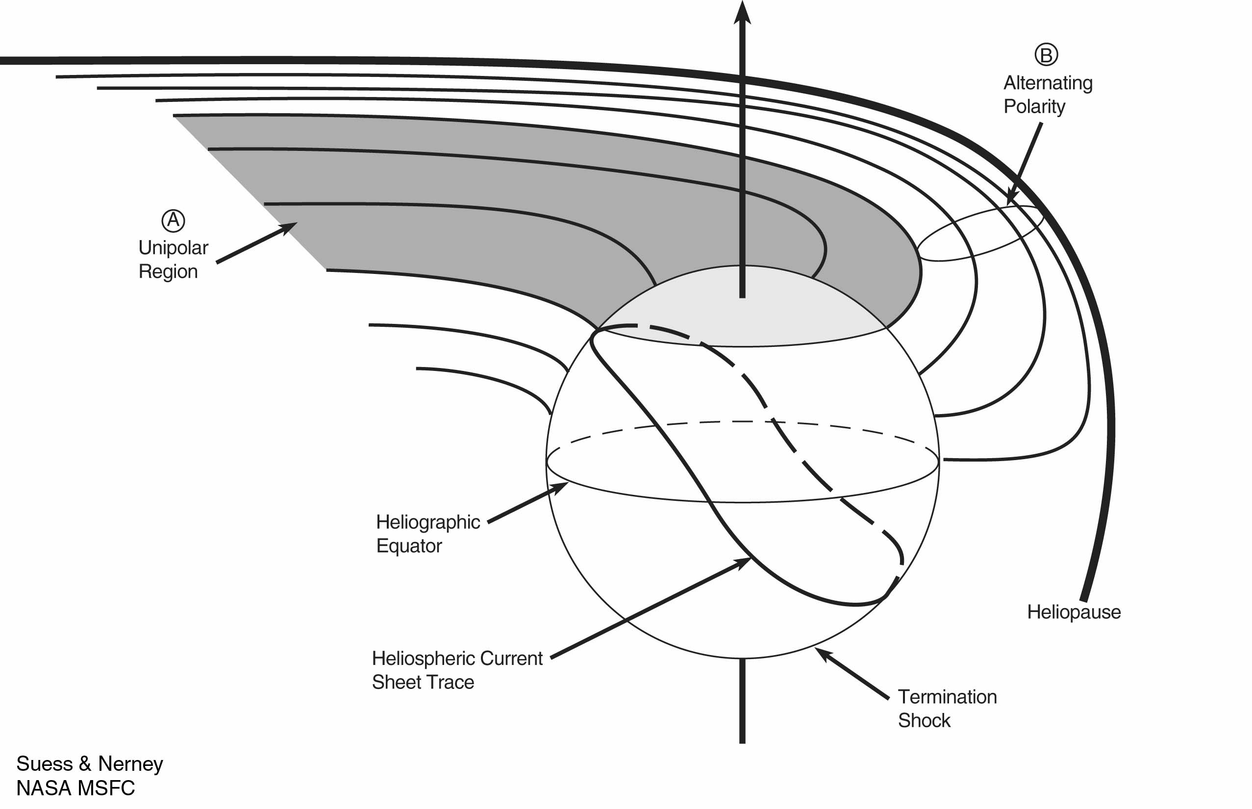
The magnetic field is amplified at the termination shock due to the slowing of the solar wind. The wind further slows as it moves outward towards the heliopause. 

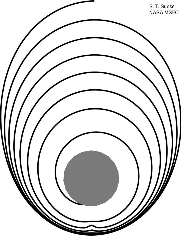
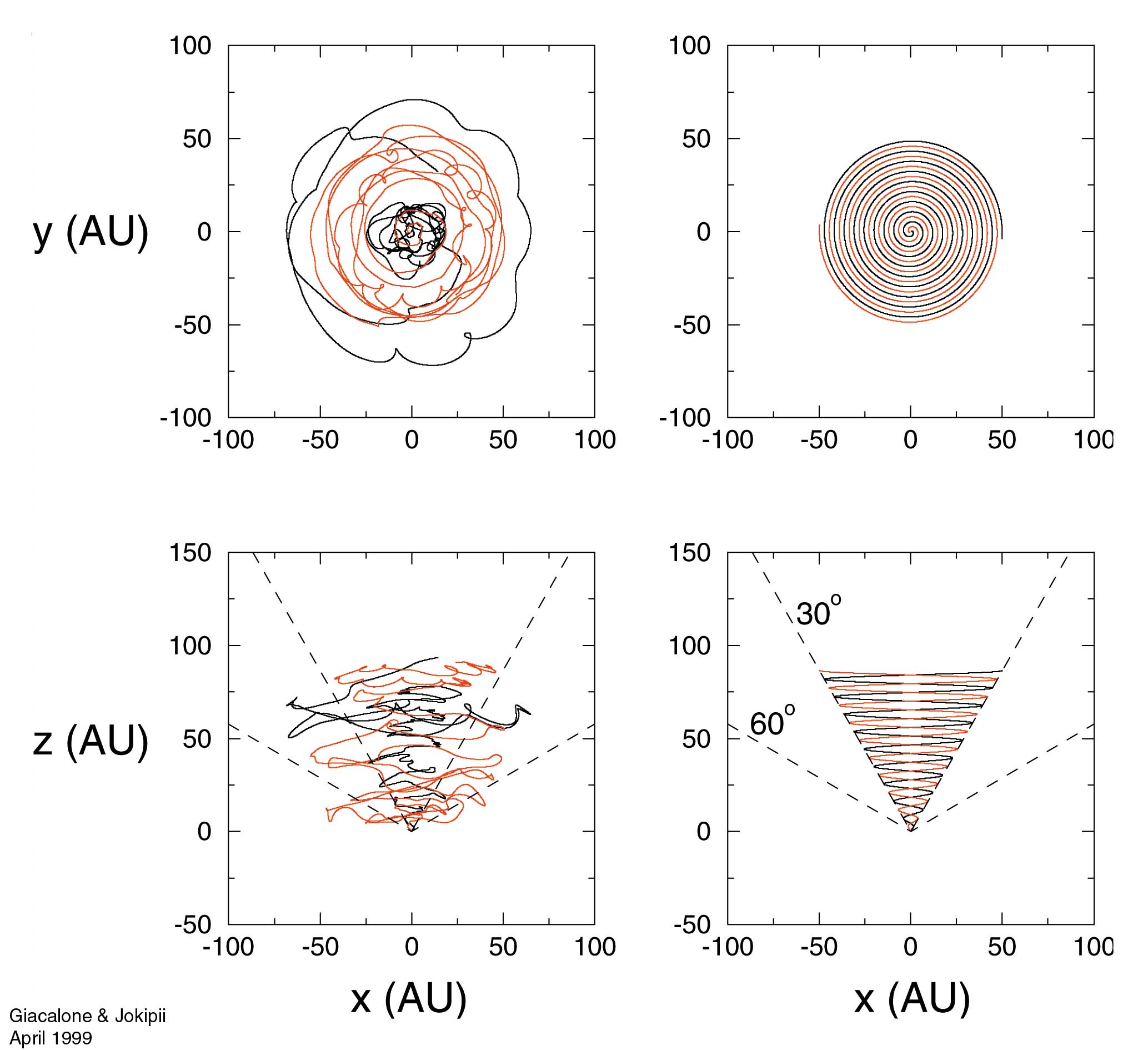
The field amplification is shown here by the more tightly spiraled magnetic field in the inner heliosheath. 

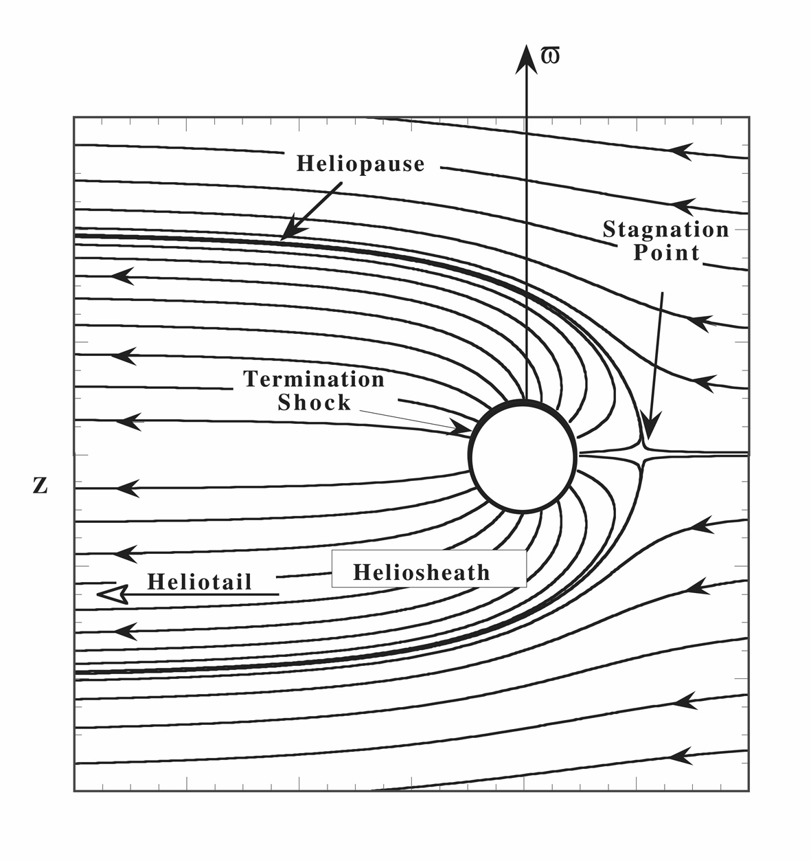
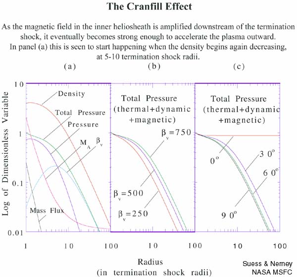
The heliospheric magnetic field is of little dynamical importance throughout most of the heliosphere. But, because of the amplification in the inner heliosheath, it is possible for the field to become strong enough to affect the flow near the stagnation point between the solar wind outflow and the incoming interstellar plasma flow, at the front of the heliopause in the upstream direction. This is called the Cranfill effect


Figure IMF.01 
(click on image for 1.39Mb jpeg)

Inner Heliosheath Flow and Advection of Magnetic Field Lines

 
Figure IMF.02
(click on image for 248Kb jpeg
   The magnetic field lines in Figure IMF.01 were computed for a spherical wind, a spherical termination shock, and no motion through the LISM. To compute the advection of the field lines around into the heliotail in detail requires a three-dimensional MHD numerical model. However, a reasonable approximation to the field line appearance can be found by assuming the field has no effect on the flow - the kinematic field approximation. The flow field shown in the Observing Objectives, reproduced here, can be used for this calculation. 

   The magnetic spirals will be centered around the solar rotation axis in IMF.02, shown by the vector v. Close to the termination shock, the spirals appear just as shown in Figure IMF.01. However, eventually the flow begins turning towards the heliotail. As this happens, the field lines also get carried tailward. This is illustrated below. 


Figure IMF.03
(click on image for 71Kb jpeg)
First consider what happens to a magnetic field line near the heliographic equator (the green line in Figure IMF.01). 

Figure IMF.03 shows a field line just 6 degrees above the equator, beginning at the termination shock - shown as the solid gray circle here. The field is compressed as the flow approaches the stagnation point, but also the field line is carried into the heliotail. This figure is shown as if viewing down from above the ecliptic plane, down along the v-axis in Figure IMF.02. 

There is a small "dimple" near the stagnation point in the upstream direction  that is due to the advection of the field line upward. This dimple is shown more clearly below. 


In the above figure, the view is from along the rotation axis of the Sun. 

Below, the same magnetic field line is shown as viewed from the side of the heliosphere, perpendicular to the upstream - downstream direction. The same magnetic field line is plotted. 

It is now apparent that the "dimple" is the dragging behind of the portion of the magnetic field line which is closest to the stagnation point and, hence, passing  through the volume with the lowest flow speeds. 

Figure IMF.04
(click image for an 81Kb gif)


These two figures show additional magnetic field lines. 

They exhibit how the tailward turning of the flow in the inner heliosheath carries magnetic field lines tailward. 

Field lines beginning at polar angles of 6 degrees (corresponding to the red line above), 30 degrees (~ the orange line), 60 degrees (~ the orange line), and 84 degrees (green line) are shown here. 

The view below is the same as that shown above. 

The view at the right is back towards the termination shock (as always, the gray sphere) from the distant heliotail. 

The nested cluster of magnetic field lines in the idealized representation is now clearly displayed. 


Figure IMF.05
(click on image for an 81Kb gif)


Figure IMF.06
(click on image for a 111Kb gif)
There is only one more aspect of the interplanetary magnetic field in the inner heliosheath that needs to be described to provide a complete description of the ideal magnetic field in the absence of any disruption downstream of the termination shock. This is the imprint of the changing polarity of the solar magnetic field. 


Cranfill Effect
 
The "Cranfill Effect" is illustrated on the right. 

These panels are prepared as if the solar wind were expanding into a perfectly still ambient interstellar medium so in the absence of a magnetic field everything would be spherically symmetric. This plot is made for the heliographic equatorial plane. The Cranfill effect can be seen in terms of the magnetic field strength across the bottom row. 
 

  • Inside the termination shock (on the left side of the thick vertical bar) the magnetic field strength falls of inversely with radius - the case for a nearly azimuthal field and constant solar wind speed. 

  •  
  • At the termination shock (assumed to be a strong shock) the field is amplified by a factor of four. 

  •  
  • Beyond the shock, the dashed lines show what the flow would be like if there were no motion through the interstellar medium. 

  •  
  • The flow speed falls off inversely with radius in this case, and the magnetic field strength increases linearly with radius.

  •  
  • Soon the magnetic field becomes strong enough to affect the flow of the plasma. When this happens, the flow speed stops dropping and the magnetic field strength quits increasing. The flow is accelerated outward by a magnetic pressure gradient force. 

  •  
  • The Cranfill Effect takes some distance to become important. For the heliosphere it is probably only important in the general vicinity of the stagnation point between solar wind flow and the interstellar flow towards the heliosphere. 

  •  
    Figure IMF.07
    (click on image for 72Kb jpeg)

     
    Figure IMF.08 shows how the Cranfill effect varies quantitatively. In particular, the panel (c) shows how it depends on polar angle. The effect is largest at the equator (90 degrees) and disappears over the poles (0 degrees). bv is the ratio of kinetic energy density to magnetic field energy density at the termination shock. MA is the Alfven Mach number. 

    Figure IMF.08

    Global MHD Model Predictions / Voyager 2 Observations
     
       Global MHD numerical models are now fully capable of making predictions for how the magnetic field will vary in the solar wind, the inner and outer heliosheaths, and on outward into the pristing interstellar medium. At the same time, there are IMF data far out into the solar system from Voyager 2. These two sources of information are combined in Figure IMF.08(a). The model curve has been normalized at the left boundary to match the Voyager data. Otherwise, the data and model are independent. 
       This model result in this figure is shown along a line in the upstream direction as defined by the motion of the heliosphere through the LISM. 
       The fall-off of the field inside the termination shock ~r-1, suggested above in Figure IMF.07, is reproduced. At the termination shock (TS), the field is amplified by the shock compression, and then continues increasing outward to the heliopause (HP). The heliopause is shifted outward due to the Cranfill effect, but the field strength does not again begin decreasing because the plot is shown in the upstream direction. 
       Beyond the heliopause, an assumption has been made that the interstellar magnetic field is 0.01 nT, transverse to the upstream direction. This provides ambient conditions appropriate for the presence of the bow shock (BS). 
    Figure IMF.08(a) 
    (click here for a postscript file)

    Field Direction Fluctuations
     
       All of the above models of the IMF made the simplifying assumption that the magnetic field at the Sun has a fixed footpoint and that the solar wind is spherically symmetric, smooth expansion. 
       At the other extreme is an assumption that leads to field lines inside the termination shock to appear as in Figure IMF.09 (compare with Figure IMF.01). 
       It is well known that magnetic flux elements in the solar photosphere random walk across the surface of the Sun. Over an interval of ~ one year, a flux element can typically random walk p/2 radians. If it assumed that footpoints of IMF lines are permanently attached to these magnetic flux elements in the photosphere then the picture at the right results. This is because it takes the solar wind ~one year to reach 1 AU. 
       Figure IMF.09 shows two field lines in the IMF, on opposite sides of the Sun but both at a latitude of 60 degrees north (polar angle of 30 degrees). On the right is shown how they would appear in the absence of a random walk of the footpoints (compare with Figure IMF.01). On the left is shown how they would appear in the presence of footpoint random walk. 

       The importance of this process is that it introduces an effective perpendicular diffusion of cosmic rays across field lines in the IMF. All cosmic ray data shows that perpendicular diffusion is important. What is not known is whether footpoint random walk is the reason for perpendicular diffusion. 

       Large transverse "Alfvenic" fluctuations have been observed to exist in the high latitude solar wind. Interstellar Probe will not address the origin of the fluctuations - Solar Probe is the correct mission for that problem. However, by making measurements of cosmic ray fluxes in radius of cosmic ray fluxes and the IMF out to the termination shock and in the inner heliosheath, the Interstellar Probe will help to solve the question of how the observed field average and statistical fluctuations produce the perpendicular diffusion. 

    Figure IMF.09
    (click on image for high-res jpeg)

    Reconnection

    Imprint of the polarity of the solar magnetic field and reconnection between the IMF and the interstellar magnetic field

       As described here, the IMF in the vicinity of the stagnation point changes polarity at least twice every solar rotation period of 25.5 days, and also fluctuates in direction due to the entrained MHD turbulence in the inner heliosheath. At the same time, the magnetic field is amplified by "pile-up" as it is carried towards the stagnation point in the upstream direction. Therefore, near the stagnation point the plasma beta (ratio of internal energy density to magnetic field energy density) is much less than one.
       At the stagnation point, the alternating polarity, low beta plasma is pressed against interstellar plasma. As is well known from conditions on the front side of the Earth's, and other planetary magnetospheres, this is precisely the condition under which reconnection will most favorably occur. It meets the two main criteria:
  • A low beta plasma in the inner heliosheath is pressed against what is probably either a low beta or O[1] beta interstellar plasma in the outer heliosheath.
  • The polarity is favorable for reconnection. The magnetic fields should be generally oppositely directed across the heliopause at the stagnation point for reconnection to take place. This is satisfied during roughly half of any given 25 day interval since the magnetic field near the equator always alternates polarity over 25 days due to solar rotation, entrained fluctuations, and the random walk of the footpoints at the Sun.
  •    Therefore, reconnection probably occurs first on the heliopause in the vicinity of the stagnation point in the upstream direction. One of the principle reasons for sending The Interstellar Probe in this direction is to have it pass through this reconnection region.
     

    Explanation

    There are two parts of the Sun's magnetic field polarity that are important for the ideal picture of the IMF in the inner heliosheath (Figures IMF.01 - IMF.08). First, the Sun's magnetic field is, to a first approximation, a tilted dipole. At latitudes equatorward of the tilt angle, the polarity changes twice every solar rotation period of 25 days. Poleward of the tilt angle, the polarity is constant over a solar rotation, but opposite in opposite hemispheres. This is depicted in Figure IMF.10. 
    Figure IMF.10
    (click on image for a 319Kb gif)
    The magnetic field of the Sun varies over the 11 year cycle of sunspot activity, and the polarity of the Sun’s magnetic field reverses at sunspot maximum. This results in a 22 year total cycle for the Sun’s magnetic field, before it returns to the beginning polarity. The imprint of the 22 year cycle is shown below. The resulting polarity "envelopes" are relatively short, in comparison to the cross-sectional size of the heliotail because the flow speed of the solar wind plasma in the inner heliosheath is extremely small. 
    Figure IMF.11
    (click image for a high-res jpeg)


    Summary

       The ideal concept of the IMF is that it is carried into smooth Archimedian spirals by the expansion of the solar wind and the rotation of the Sun. Interplanetary observations show that this picture is obtained only after averaging IFM data - generally over a full solar rotation. There are many superimposed Alfvenic fluctuations which grow in amplitude with increasing heliocentric distance. There may also be footpoint random walk of the field lines at the Sun.
       In the inner heliosheath, the IMF is turned and carried into the heliotail. It is also compressed and amplified as the flow slows to turn tailward. This leads to the possibility of MHD forces being important in inner heliosheath flow.
       Near the stagnation point conditions are ideal for reconnection to take place between the IMF and the interstellar magnetic field. Generally reconnection is observed to be sporadic, accelerate particles to cosmic ray energies, and to generate radio waves. All this will be observed in situ with the Interstellar Probe.
     

    Return to Introduction
    Return to Observing Objectives
    Return to Mission Technology