ISP-ObservObj.html

Return to Introduction
Go to Mission Technology Observing Objectives

The Scientific Objectives listed in the Introduction are designed to produce a much more detailed picture of the heliosphere and what it looks like. They will specifically produce answers on the shape of the termination shock and on the thickness of both the inner and outer heliosheaths.

The Scientific Objectives lead to a group of Observing Objectives. These are a detailed description of what phenomena will be measured at what distances from the Sun, and where the measurements are most important.

Figure OO.01
(Click on image for a 256Kb jpeg)
(click here for a postscript file)

Terminology in Observing Objectives Figure

TS: Termination shock
HP: Heliopause
BS: Bow shock - which exists only if external flow is supersonic and superAlfvenic

Purple horizontal arrow: Marks the upstream direction of the motion of the heliosphere through the local interstellar medium and is the approximate direction that The Interstellar Probe will travel.

Observing Objectives - Explanations & Details

Refer to the horizontal bars on page 6 for identification of the Observing Objectives and where the observations will be concentrated. (follow links below to details on the phenomena)

Heliosheath Solar Wind Plasma

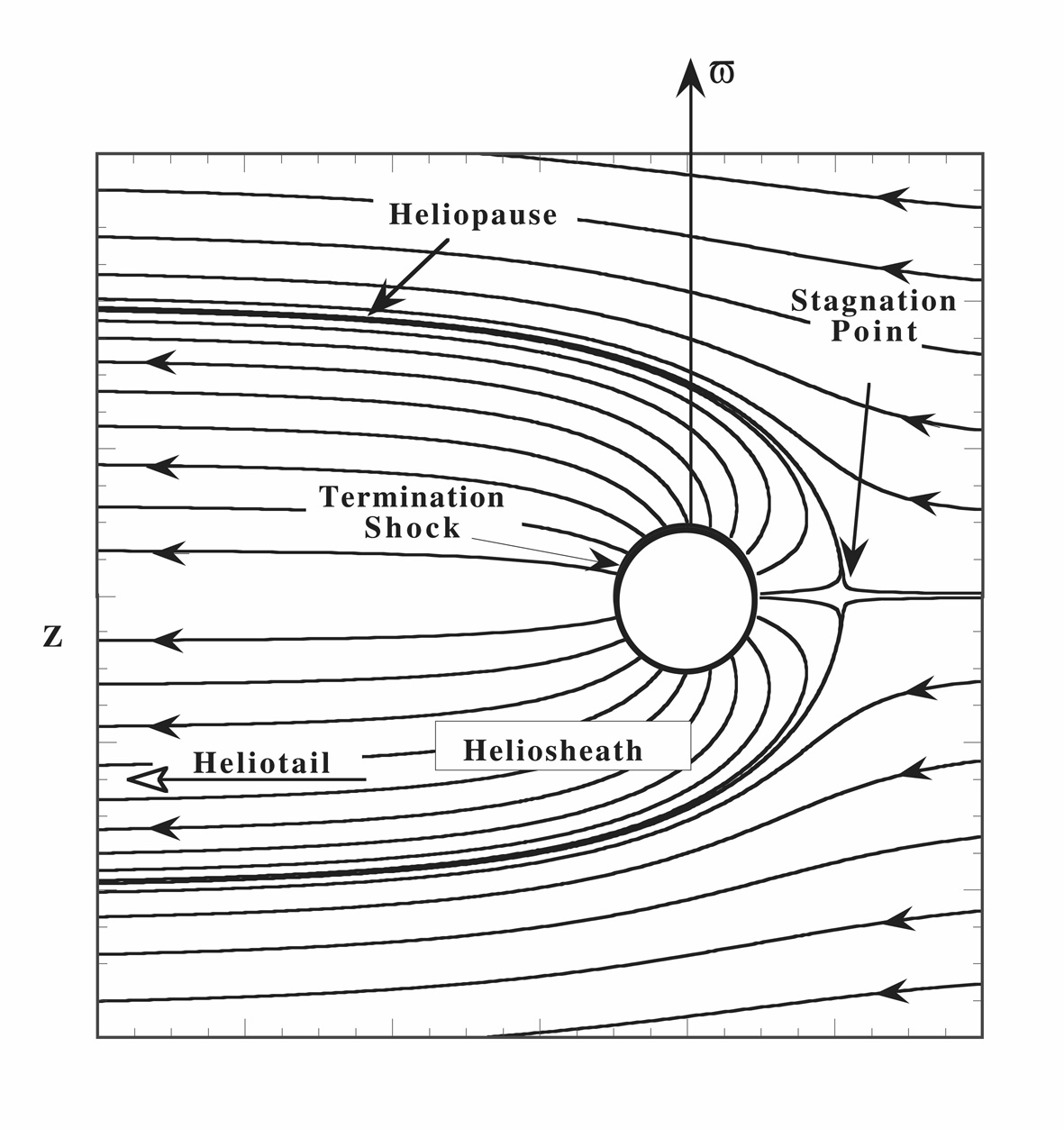
Solar wind plasma expands more-or-less freely until it meets the local interstellar medium (LISM). On the simplest level, the interaction is stagnation point flow between two fluids flowing towards each other. In the example shown here, there is a spherical source (the Sun) of outflow and a planar flow from the right. Both flows come to a halt (in the solar frame of reference) at the stagnation point. As the flows approach the stagnation point, they are turned. The LISM flow dominates so it forces the solar wind to turn and eventually flow in the same direction as the LISM flow, down the heliotail. The surface that divides the two flows is the heliopause.

Solar wind flow is initially supersonic. Therefore, it will generally have to be slowed before it can be turned to flow down the heliotail. Solar wind flow normally will slow abruptly at the termination shock, with supersonic flow inside the termination shock and subsonic flow outside the termination shock - in the inner heliosheath. The termination shock is thought to be at ~100 AU.

The direction of solar north (solar rotation) is indicated here by v. However, the ideal situation shown here is axisymmetric about the axis in the LISM upstream direction.

As solar wind plasma passes through the termination shock it is heated back to coronal temperatures of ~one million degrees. It is also compressed by a factor of <~ four, although the density is so small at 100 AU that the compression still leaves a very sparse plasma of less than one particle per cubic centimeter (0.1 - 0.3 per cubic centimeter).

The flow speed just inside the termination shock is 400-750 km/s and 100-200 km/s just beyond the termination shock. This decreases as the flow is turned and the flow speed in heliotail is ~25 km/s.

If the LISM flow speed is faster than the sound and Alfven speeds then there will also be a bow shock out in front of the stagnation point. In this case, there will also be an outer heliosheath between the heliopause and the bow shock.

Figure OO.02
(click on image for 248Kb jpeg)

Measurement Objectives:

Plasma density

Plasma temperature

Plasma anisotropies

Plasma flow vector

Plasma statistical fluctuations

Plasma thermal flux

Web site:

Timur Linde modeling pictures: http://hpcc.engin.umich.edu/HPCC/recent2/index.html

Interplanetary Magnetic Field (click on title to go to detailed discussion)

The interplanetary magnetic field (IMF) is drawn into a Archimedian spirals as it is carried away from the Sun by the solar wind. This happens because the footpoints of the field remain attached to the Sun, which is rotating once every 25.5 days. Since it takes on the order of one year for the solar wind to reach the termination shock, 10-20 complete spirals are formed over this distance. These spirals are shown in Figure OO.02 for three magnetic field lines at solar latitudes of 6, 45, and 84 degrees north (green, orange, and red, respectively).

At the termination shock the IMF is amplified in exactly the same way the solar wind plasma is compressed. Beyond the termination shock the IMF is further amplified as the solar wind in the inner heliosheath is slowed and turned. The field amplification is shown here by the more tightly spiraled magnetic field in the inner heliosheath.

Figure OO.02 is highly idealized because it neglects several phenomena which might otherwise mask or even obliterate the perfect spirals illustrated here. These phenomena include, but are not limited to, footpoint wandering at the Sun due to convective motions in the photosphere and turbulent fluctuations introduced in the corona, solar wind, and at the termination shock.

Measurement Objectives:

Field strength

Field direction

Field statistical properties

Figure OO.03
(click on image for 1.39Mb jpeg)
(click on this line for a postscript file)

Cranfill Effect

The heliospheric magnetic field is of little dynamical importance throughout most of the heliosphere. But, because of the amplification in the inner heliosheath, it is possible for the field to become strong enough to affect the flow near the stagnation point between the solar wind outflow and the incoming interstellar plasma flow, at the front of the heliopause in the upstream direction. This is called the Cranfill effect.

Measurement Objectives:

Plasma beta (ratio of internal energy density to magnetic field energy density)

Ratio of kinetic energy density to magnetic field energy density

Distance to the heliopause

Field Direction Fluctuations

Even inside the termination shock, the IMF is not ever smooth. Fluctuations in direction occur on all time scales down to far less than one second. At times longer than a day, the fluctuations are primarily due to changes in the dominant polarity at the Sun and are discussed below in relation to reconnection. At shorter time scales, the fluctuations are due to:

The movement of field line footpoints around the surface of the Sun. This concept is a random walk process due to convection in the photosphere. It is important to the degree that IMF field lines remain attached to the same flux element at their footpoints for more than a few hours.
Fluctuations due to MHD turbulence introduced in the corona, between the photosphere and 10-30 solar radii.
Fluctuations introduced at the termination shock.

These fluctuations affect the propagation of cosmic rays throughout the heliosphere. The scattering of cosmic rays by the fluctuations produces an effective diffusion of the cosmic rays across magnetic field lines. Such diffusion is known to exist and be much larger than predicted by classical (smooth IMF) theory.

Measurement Objectives:

Statistics of the IMF between time scales of a fraction of a second and a few months.

Reconnection

The IMF in the vicinity of the stagnation point changes polarity at least twice every solar rotation period of 25.5 days, and also fluctuates in direction due to the entrained MHD turbulence in the inner heliosheath. At the same time, the magnetic field is being amplified by "pile-up" as it is carried towards the stagnation point in the upstream direction. Therefore, near the stagnation point the plasma beta (ratio of internal energy density to magnetic field energy density) is much less than one.
At the stagnation point, the alternating polarity, low beta plasma is pressed against interstellar plasma. As is well known from conditions on the front side of the Earth's, and other planetary magnetospheres, this is precisely the condition under which reconnection will most favorably occur. It meets the two main criteria:

A low beta plasma in the inner heliosheath is pressed against what is probably either a low beta or O[1] beta interstellar plasma in the outer heliosheath.

The polarity being favorable for reconnection. The magnetic fields should be generally oppositely directed across the heliopause at the stagnation point for reconnection to take place. This is satisfied during roughly half of any given 25 day interval since the magnetic field near the equator always alternates polarity over 25 days due to solar rotation and fluctuates continuously in direction.

Therefore, reconnection probably occurs first on the heliopause in the vicinity of the stagnation point in the upstream direction. One of the principle reasons for sending The Interstellar Probe in this direction is to have it pass through this reconnection region.

Measurement Objectives:

Energetic particles streaming upstream towards the Sun, away from the stagnation point, in the inner heliosheath.

Radio noise originating from the vicinity of the stagnation point.

Anomalous Cosmic Rays

In the anomalous component of cosmic rays, fluxes of helium, nitrogen, oxygen, neon, protons, and carbon are observed to be enhanced in a region of the energy spectrum ranging from a kinetic energy of 20 MeV to ~300 MeV. The radial intensity gradient of these particles is positive out to the maximum distance reached by current spacecraft, indicating that this component is not of solar origin, an that it probably originates in the outer solar system. It is likely that anomalous cosmic rays are particles in the solar wind that are accelerated at the termination shock. The particles in the solar wind are not, however, ambient solar wind plasma. instead, the particles are initially neutral interstellar atoms that have streamed into the heliosphere as a consequence of its motion through the LISM. They have become ionized and picked up by the solar wind and then carried with the IMF back out to the termination shock. There they are accelerated to the observed energies. It was predicted that the particles would be predominantly in a charge state of +1 if the hypothesis for their origin were correct and this has recently been confirmed.
Interstellar probe would determine the radial gradient, composition, and spectra of anomalous cosmic rays outward to the termination shock, where they originate, and then outward from there to distances where their influence is virtually absent (anticipated to be beyond ~300 AU).

Measurement Objectives:

Anomalous cosmic rays fluxes and energy spectra

Anomalous cosmic ray composition

Pickup Ions

Interstellar neutral gas flows relatively unimpeded into the heliosphere, although it possibly experiences filtration at the heliospheric boundaries. Neutral interstellar hydrogen is especially susceptible to the effects of filtration, being decelerated and heated in passing from the LISM into the heliosphere. Atoms flowing into the supersonic solar wind inside the termination shock can undergo either photoionization or charge exchange ionization and the new ions almost instantaneously respond to the electromagnetic fields in the solar wind. The newly born ions immediately gyrate about the IMF, after which they experience scattering and isotropization by either ambient or self-generated low-frequency electromagnetic fluctuations in the solar wind plasma. Since the newly born ions are eventually isotropized, their mean bulk velocity is now that of the solar wind i.e., they convect with the solar wind flow, and are then said to be picked up by the solar wind. The isotropized pickup ions form a distinct population of energetic ions (~1 KeV) in the solar wind whose origin is the interstellar medium and which serves as the seed population for anomalous cosmic rays.

Neutral Hydrogen UV Glow

Neutral Hydrogen UV Glow

Zodiacal Light

Zodiacal light
http://spider.ipac.caltech.edu/staff/reach/figures/band.html

Kuiper Belt Dust

There are at at least 70,000 trans-Neptunian objects in the outer solar system with diameters larger than 100 km in the radial zone extending outwards from the orbit of Neptune (at 30 AU) to 50 AU. There may be many more bodies beyond 50 Au, but these are presently beyond the limits of detection. Observations show that the trans-Neptunians are mostly confined within a few degrees of the ecliptic, leading to the realization that they occupy a ring or belt surrounding the Sun. This ring is generally referred to as the Kuiper Belt.
The Kuiper Belt holds significance for the study of the planetary system on at least two levels. First, it is likely that Kuiper Belt objects are extremely primitive remnants from the early accretional phases of the solar system. The inner, dense parts of the pre-planetary disk condensed into the major planets, probably within a few millions to tens of millions of years. The outer parts were less dense, and accretion progressed slowly. Evidently, a great many small objects were formed. Second, it widely believed that the Kuiper Belt is the source of short period comets.
Kuiper belt dust
http://www.ifa.hawaii.edu/faculty/jewitt/kb.html

Energetic Neutral Atoms

Energetic neutral atoms

Pileup (H, Ions, Dust, Interstellar Magnetic Field)

Pileup

Hydrogen Wall

Hydrogen wall

Interstellar Magnetic Field

Interstellar magnetic field

Isotopic Composition and Properties of Interstellar Plasma - p+, e-, C, N, O, Fe ions, etc.

Isotopic Composition of Interstellar Neutral Atoms

Interstellar Neutrals - H, D, He, N, O, etc.

High Energy Cosmic Rays

Low Energy Cosmic Rays

Filtration (H, O, Dust)

Large Interstellar Dust Grains

Dust grains in the diffuse inerstellar medium have been believed to be smaller than 0.5 microns until larger ones have been discovered by the dust detectors on-board the interplanetary spacecraft Ulysses and Galileo. Since large grains are much less abundant than small interstellar dust grains, they do not contribute much to the extinction of starlight and are thus hard to observe spectroscopically. Therefore, in-situ measurements are needed to measure the flux and/or composition of the large-grain component in interstellar space. Despite their low spatial concentration, large interstellar grains carry a large fraction of the total dust mass in the local interstellar medium, and potentially distribute large amounts of refratory/organic substances over large spatial scales.

Large intersellar grains penetrate the heliopause unperturbed due to their large inertia. They move in good approximation on hyperbolic trajectories through the heliosphere. The bending of the grain's trajectories towards the Sun causes their spatial density to be enhanced in a regeion downstream of the Sun. This region is called the gravitational focus and is shaped like a parabola. The picture on the right shows the calculated spatial distribution of large interstellar grains in a 20AU x 20AU plane around the Sun. The grains enter the plane from the right and move to the left. The gravitational focus is clearly visible on the right hand side of the picture.

(click on image to enlarge)

This is what a interstellar dust particle might look like. Many such dust grains are collected in the upper atmosphere by aircraft flying at high altitudes. Most of these grains are believed to be interplanetary dust grains (IDPs), but grains have been found inside the IDPs that show non-solar isotopic composition. Top candidates for interstellar grains are GEMS (glass with embedded metals and sulfides) that consist mainly of amorphous silicate, which is also believed to be the major constituent of interstellar dust grains. GEMS are typically some tenths of a micron to some micron in size, and are therefore larger than "classical interstellar grains". A collection of IDPs is kept at the Astromaterial Collection Facility at the NASA Johnson Space Center.

Small Interstellar Dust Grains

Extinction of starlight in the EUV indicates that solid particles in interstellar space can be as small as large mono-molecules. A good fit to the spectroscopic data is achieved when considering polycyclic aromatic hydrocarbon (PAH) molecules. The largest grains that are evident from extinction measurements have diameter of about 0.5 microns. This size range can be considered as "classical" interstellar grains, because their existence was known long before the in-situ measurements of interstellar grains in the Solar System. Fits to the extinction curve indicate that the grain size distribution drops very steep to large masses, that is, small interstellar grains are much more abundant than large ones. If this is true, why haven't they been discovered in early in-situ measurements (e.g. with the instruments on-board the Pioneer 8 and 9 spacecraft)? After the obvious non-detection of interstellar dust by Pionner, it was argued that the grains develop a electrostatic charge in the plasma and radiation environment of interplanetary space, and that this charge couples them to the solar wind, which transports them out of the Solar System. This interpretation is consistent with the mass distribution of interstellar grains that have been detected in-situ by Ulyssess and Galileo.

Modeling the motion of small interstellar dust particles through the heliopause has shown that the solar wind magnetic field is capable of inhibiting small grains from entering the inner Solar System. The figure on the right shows the spatial distribuion of 0.1 micron grains that enter the Solar System from the right with a velocity of 26 km/s. The panel covers an area of 80AU x 80AU. The actual distribution depends on the phase of the solar cycle, since the magnetic field polarity in the solar wind changes with the cycle. As a result of the deceleration of the grains, a region of increased spatial density forms upstream of the Sun. The spatial density inside 5AU is strongly reduced during the whole 22-year solar cycle.

(click on image to enlarge)

Recently, it was argued, that grains in the size range below 0.05 microns can interact strongly with the compressed magnetic field in the heliopause region, effectively diverting them around the heliosphere. Unfortunately, such small grains are out of the sensitivity range of todays in-situ dust detectors. Outside the heliosphere interstellar grains of sizes of a few tens of a nanometer should be present abundantly, as indicated by the extinction data. One very interesting quantity to measure in interstellar space is the velocity dispersion of these small grains, since the dispersion indicates the amount of disturbance that the local cloud has experienced in the past.

Return to Introduction
Go to Mission Technology